Display glacier area and thickness changes on a grid#
from oggm import cfg
from oggm import tasks, utils, workflow, graphics, DEFAULT_BASE_URL
import salem
import xarray as xr
import numpy as np
import glob
import os
import matplotlib.pyplot as plt
This notebook proposes a method for redistributing glacier ice that has been simulated along the flowline after a glacier retreat simulation. Extrapolating the glacier ice onto a map involves certain assumptions and trade-offs. Depending on the purpose, different choices may be preferred. For example, higher resolution may be desired for visualization compared to using the output for a hydrological model. It is possible to add different options to the final function to allow users to select the option that best suits their needs.
This notebook demonstrates the redistribution process using a single glacier. Its purpose is to initiate further discussion before incorporating it into the main OGGM code base (currently, it is in the sandbox).
Pick a glacier#
# Initialize OGGM and set up the default run parameters
cfg.initialize(logging_level='WARNING')
# Local working directory (where OGGM will write its output)
# WORKING_DIR = utils.gettempdir('OGGM_distr4')
cfg.PATHS['working_dir'] = utils.get_temp_dir('OGGM_distributed', reset=True)
2026-07-20 12:59:56: oggm.cfg: Reading default parameters from the OGGM `params.cfg` configuration file.
2026-07-20 12:59:56: oggm.cfg: Multiprocessing switched OFF according to the parameter file.
2026-07-20 12:59:56: oggm.cfg: Multiprocessing: using all available processors (N=4)
rgi_ids = ['RGI60-11.01450', # Aletsch
'RGI60-11.01478'] # Fieschergletscher
gdirs = workflow.init_glacier_directories(rgi_ids, prepro_base_url=DEFAULT_BASE_URL, from_prepro_level=4, prepro_border=80)
2026-07-20 12:59:57: oggm.workflow: init_glacier_directories from prepro level 4 on 2 glaciers.
2026-07-20 12:59:57: oggm.workflow: Execute entity tasks [gdir_from_prepro] on 2 glaciers
Experiment: a random warming simulation#
Here we use a random climate, but you can use any GCM, as long as glaciers are getting smaller, not bigger!
# Do a random run with a bit of warming
workflow.execute_entity_task(
tasks.run_random_climate,
gdirs,
ys=2020, ye=2100, # Although the simulation is idealised, lets use real dates for the animation
y0=2009, halfsize=10, # Random climate of 1999-2019
seed=1, # Random number generator seed
temperature_bias=1.5, # additional warming - change for other scenarios
store_fl_diagnostics=True, # important! This will be needed for the redistribution
init_model_filesuffix='_spinup_historical', # start from the spinup run
output_filesuffix='_random_s1', # optional - here I just want to make things explicit as to which run we are using afterwards
);
2026-07-20 12:59:58: oggm.workflow: Execute entity tasks [run_random_climate] on 2 glaciers
Redistribute: preprocessing#
The required tasks can be found in the distribute_2d module of the sandbox:
from oggm.sandbox import distribute_2d
# This is to add a new topography to the file (smoothed differently)
workflow.execute_entity_task(distribute_2d.add_smoothed_glacier_topo, gdirs)
# This is to get the bed map at the start of the simulation
workflow.execute_entity_task(tasks.distribute_thickness_per_altitude, gdirs)
# This is to prepare the glacier directory for the interpolation (needs to be done only once)
workflow.execute_entity_task(distribute_2d.assign_points_to_band, gdirs);
2026-07-20 12:59:59: oggm.workflow: Execute entity tasks [add_smoothed_glacier_topo] on 2 glaciers
2026-07-20 12:59:59: oggm.workflow: Execute entity tasks [distribute_thickness_per_altitude] on 2 glaciers
2026-07-20 13:00:00: oggm.workflow: Execute entity tasks [assign_points_to_band] on 2 glaciers
Let’s have a look at what we just did:
gdir = gdirs[0] # here for Aletsch
#gdir = gdirs[1] # uncomment for Fieschergletscher
with xr.open_dataset(gdir.get_filepath('gridded_data')) as ds:
ds = ds.load()
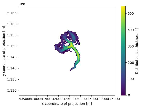
# Initial glacier thickness
f, ax = plt.subplots()
ds.distributed_thickness.plot(ax=ax)
ax.axis('equal');
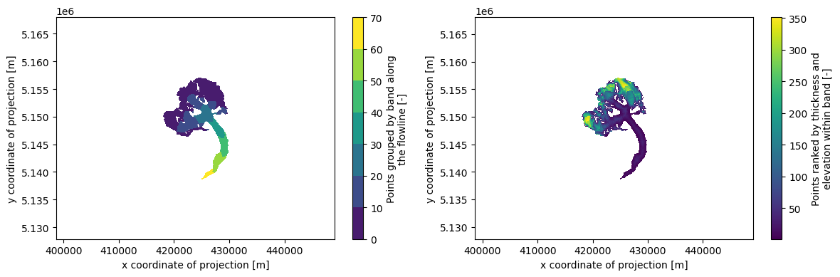
# Which points belongs to which band, and then within one band which are the first to melt
f, (ax1, ax2) = plt.subplots(1, 2, figsize=(12, 4))
ds.band_index.plot.contourf(ax=ax1)
ds.rank_per_band.plot(ax=ax2)
ax1.axis('equal'); ax2.axis('equal'); plt.tight_layout();
Redistribute simulation#
The tasks above need to be run only once. The next one however should be done for each simulation:
ds = workflow.execute_entity_task(
distribute_2d.distribute_thickness_from_simulation,
gdirs,
input_filesuffix='_random_s1', # Use the simulation we just did
concat_input_filesuffix='_spinup_historical', # Concatenate with the historical spinup
output_filesuffix='', # filesuffix added to the output filename gridded_simulation.nc, if empty input_filesuffix is used
)
2026-07-20 13:00:01: oggm.workflow: Execute entity tasks [distribute_thickness_from_simulation] on 2 glaciers
/usr/local/pyenv/versions/3.13.13/lib/python3.13/site-packages/oggm/utils/_workflow.py:522: SerializationWarning: saving variable time with floating point data as an integer dtype without any _FillValue to use for NaNs
out = task_func(gdir, **kwargs)
/usr/local/pyenv/versions/3.13.13/lib/python3.13/site-packages/oggm/utils/_workflow.py:522: SerializationWarning: saving variable time with floating point data as an integer dtype without any _FillValue to use for NaNs
out = task_func(gdir, **kwargs)
Plot#
Let’s have a look!
# # This below is only to open the file again later if needed
# with xr.open_dataset(gdir.get_filepath('gridded_simulation', filesuffix='_random_s1')) as ds:
# ds = ds.load()
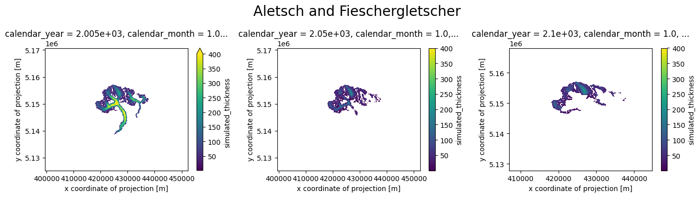
def plot_distributed_thickness(ds, title):
f, (ax1, ax2, ax3) = plt.subplots(1, 3, figsize=(14, 4))
ds.simulated_thickness.sel(time=2005).plot(ax=ax1, vmax=400)
ds.simulated_thickness.sel(time=2050).plot(ax=ax2, vmax=400)
ds.simulated_thickness.sel(time=2100).plot(ax=ax3, vmax=400)
ax1.axis('equal'); ax2.axis('equal'); f.suptitle(title, fontsize=20)
plt.tight_layout();
plot_distributed_thickness(ds[0], 'Aletsch')
# plot_distributed_thickness(ds[1], 'Fieschergletscher')
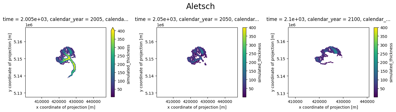
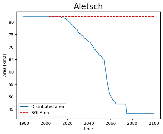
Note: the simulation before the RGI date cannot be trusted - it is the result of the dynamical spinup. Furthermore, if the area is larger than the RGI glacier, the redistribution algorithm will put all mass in the glacier mask, which is not what we want:
def plot_area(ds, gdir, title):
area = (ds.simulated_thickness > 0).sum(dim=['x', 'y']) * gdir.grid.dx**2 * 1e-6
area.plot(label='Distributed area')
plt.hlines(gdir.rgi_area_km2, gdir.rgi_date, 2100, color='C3', linestyles='--', label='RGI Area')
plt.legend(loc='lower left'); plt.ylabel('Area [km2]'); plt.title(title, fontsize=20); plt.show();
plot_area(ds[0], gdirs[0], 'Aletsch')
# plot_area(ds[1], gdirs[1], 'Fieschergletscher')
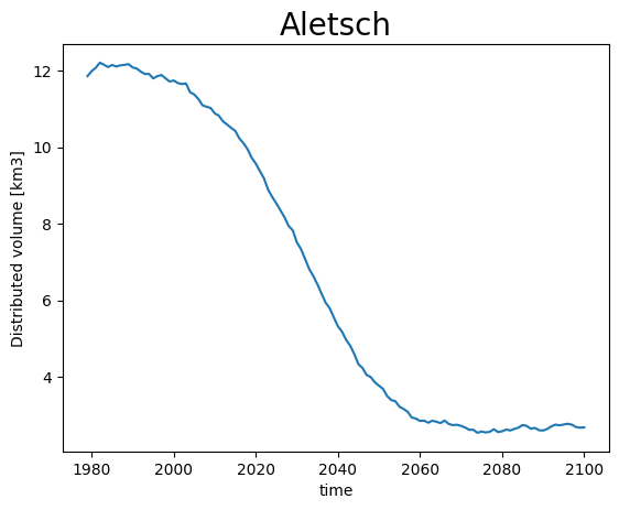
Volume however is conserved:
def plot_volume(ds, gdir, title):
vol = ds.simulated_thickness.sum(dim=['x', 'y']) * gdir.grid.dx**2 * 1e-9
vol.plot(label='Distributed volume'); plt.ylabel('Distributed volume [km3]')
plt.title(title, fontsize=20); plt.show();
plot_volume(ds[0], gdirs[0], 'Aletsch')
# plot_volume(ds[1], gdirs[1], 'Fieschergletscher')
Therefore, lets just keep all data after the RGI year only:
for i, (ds_single, gdir) in enumerate(zip(ds, gdirs)):
ds[i] = ds_single.sel(time=slice(gdir.rgi_date, None))
Animation!#
from matplotlib import animation
from IPython.display import HTML
# Get a handle on the figure and the axes
fig, ax = plt.subplots()
thk = ds[0]['simulated_thickness'] # Aletsch
# thk = ds[1]['simulated_thickness'] # Fieschergletscher
# Plot the initial frame.
cax = thk.isel(time=0).plot(ax=ax,
add_colorbar=True,
cmap='viridis',
vmin=0, vmax=thk.max(),
cbar_kwargs={
'extend':'neither'
}
)
ax.axis('equal')
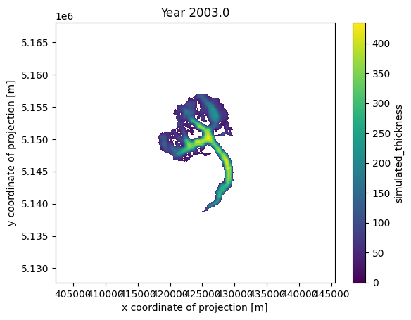
def animate(frame):
ax.set_title(f'Year {int(thk.time[frame])}')
cax.set_array(thk.values[frame, :].flatten())
ani_glacier = animation.FuncAnimation(fig, animate, frames=len(thk.time), interval=100);

HTML(ani_glacier.to_jshtml())
# Write to mp4?
# FFwriter = animation.FFMpegWriter(fps=10)
# ani2.save('animation.mp4', writer=FFwriter)
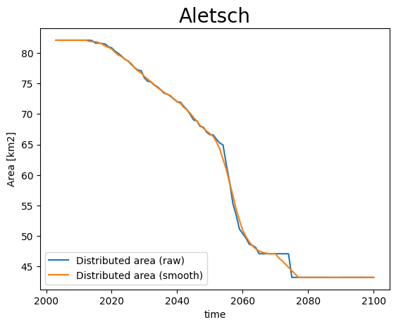
Finetune the visualisation#
When applying the tools you might see that sometimes the timeseries are “shaky”, or have sudden changes in area. This comes from a few reasons:
OGGM does not distinguish between ice and snow, i.e. when it snows a lot sometimes OGGM thinks there is a glacier for a couple of years.
the trapezoidal flowlines result in sudden (“step”) area changes when they melt entirely.
on small glaciers, the changes within one year can be big, and you may want to have more intermediate frames
We implement some workarounds for these situations:
ds_smooth = workflow.execute_entity_task(
distribute_2d.distribute_thickness_from_simulation,
gdirs,
input_filesuffix='_random_s1',
concat_input_filesuffix='_spinup_historical',
ys=2003, ye=2100, # make the output smaller
output_filesuffix='_random_s1_smooth', # do not overwrite the previous file (optional)
# add_monthly=True, # more frames! (12 times more - we comment for the demo, but recommend it)
rolling_mean_smoothing=7, # smooth the area time series
fl_thickness_threshold=1, # avoid snow patches to be misclassified
)
2026-07-20 13:00:19: oggm.workflow: Execute entity tasks [distribute_thickness_from_simulation] on 2 glaciers
/usr/local/pyenv/versions/3.13.13/lib/python3.13/site-packages/oggm/utils/_workflow.py:522: SerializationWarning: saving variable time with floating point data as an integer dtype without any _FillValue to use for NaNs
out = task_func(gdir, **kwargs)
/usr/local/pyenv/versions/3.13.13/lib/python3.13/site-packages/oggm/utils/_workflow.py:522: SerializationWarning: saving variable time with floating point data as an integer dtype without any _FillValue to use for NaNs
out = task_func(gdir, **kwargs)
def plot_area_smoothed(ds_smooth, ds, gdir, title):
area = (ds.simulated_thickness > 0).sum(dim=['x', 'y']) * gdir.grid.dx**2 * 1e-6
area.plot(label='Distributed area (raw)')
area = (ds_smooth.simulated_thickness > 0).sum(dim=['x', 'y']) * gdir.grid.dx**2 * 1e-6
area.plot(label='Distributed area (smooth)')
plt.legend(loc='lower left'); plt.ylabel('Area [km2]')
plt.title(title, fontsize=20); plt.show();
plot_area_smoothed(ds_smooth[0], ds[0], gdirs[0], 'Aletsch')
# plot_area_smoothed(ds_smooth[1], ds[1], gdirs[1], 'Fieschergletscher')
# Get a handle on the figure and the axes
fig, ax = plt.subplots()
thk = ds_smooth[0]['simulated_thickness'] # Aletsch
# thk = ds_smooth[1]['simulated_thickness'] # Fieschergletscher
# Plot the initial frame.
cax = thk.isel(time=0).plot(ax=ax,
add_colorbar=True,
cmap='viridis',
vmin=0, vmax=thk.max(),
cbar_kwargs={
'extend':'neither'
}
)
ax.axis('equal')
def animate(frame):
ax.set_title(f'Year {float(thk.time[frame]):.1f}')
cax.set_array(thk.values[frame, :].flatten())
ani_glacier = animation.FuncAnimation(fig, animate, frames=len(thk.time), interval=100);
# Visualize
HTML(ani_glacier.to_jshtml())
# Write to mp4?
# FFwriter = animation.FFMpegWriter(fps=120)
# ani2.save('animation_smooth.mp4', writer=FFwriter)
Merge redistributed thickness from multiple glaciers#
If you’re working in a region with multiple glaciers, displaying the evolution of all glaciers simultaneously can be convenient. To facilitate this, we offer a tool that merges the simulated distributed thicknesses of multiple glaciers.
This process can be very memory-intensive. To prevent memory overflow issues, we, by default, merge the data for each year into a separate file. If you have sufficient resources, you can set save_as_multiple_files=False to compile the data into a single file at the end. However, with xarray.open_mfdataset, you have the capability to seamlessly open and work with these multiple files as if they were one.
For further explanation on merging gridded_data, please consult the tutorial Ingest gridded products such as ice velocity into OGGM.
simulation_filesuffix = '_random_s1_smooth' # saved in variable for later opening of the files
distribute_2d.merge_simulated_thickness(
gdirs, # the gdirs we want to merge
simulation_filesuffix=simulation_filesuffix, # the name of the simulation
years_to_merge=np.arange(2005, 2101, 5), # for demonstration, I only pick some years, if this is None all years are merged
add_topography=True, # if you do not need topography setting this to False will decrease computing time
preserve_totals=True, # preserve individual glacier volumes during merging
reset=True,
)
2026-07-20 13:00:35: oggm.sandbox.distribute_2d: Applying global task merge_simulated_thickness on 2 glaciers
2026-07-20 13:00:35: oggm.workflow: Applying global task merge_gridded_data on 2 glaciers
2026-07-20 13:00:37: oggm.workflow: Applying global task merge_gridded_data on 2 glaciers
2026-07-20 13:00:37: oggm.workflow: Applying global task merge_gridded_data on 2 glaciers
2026-07-20 13:00:37: oggm.workflow: Applying global task merge_gridded_data on 2 glaciers
2026-07-20 13:00:38: oggm.workflow: Applying global task merge_gridded_data on 2 glaciers
2026-07-20 13:00:38: oggm.workflow: Applying global task merge_gridded_data on 2 glaciers
2026-07-20 13:00:38: oggm.workflow: Applying global task merge_gridded_data on 2 glaciers
2026-07-20 13:00:38: oggm.workflow: Applying global task merge_gridded_data on 2 glaciers
2026-07-20 13:00:38: oggm.workflow: Applying global task merge_gridded_data on 2 glaciers
2026-07-20 13:00:38: oggm.workflow: Applying global task merge_gridded_data on 2 glaciers
2026-07-20 13:00:39: oggm.workflow: Applying global task merge_gridded_data on 2 glaciers
2026-07-20 13:00:39: oggm.workflow: Applying global task merge_gridded_data on 2 glaciers
2026-07-20 13:00:39: oggm.workflow: Applying global task merge_gridded_data on 2 glaciers
2026-07-20 13:00:39: oggm.workflow: Applying global task merge_gridded_data on 2 glaciers
2026-07-20 13:00:39: oggm.workflow: Applying global task merge_gridded_data on 2 glaciers
2026-07-20 13:00:39: oggm.workflow: Applying global task merge_gridded_data on 2 glaciers
2026-07-20 13:00:39: oggm.workflow: Applying global task merge_gridded_data on 2 glaciers
2026-07-20 13:00:40: oggm.workflow: Applying global task merge_gridded_data on 2 glaciers
2026-07-20 13:00:40: oggm.workflow: Applying global task merge_gridded_data on 2 glaciers
2026-07-20 13:00:40: oggm.workflow: Applying global task merge_gridded_data on 2 glaciers
2026-07-20 13:00:40: oggm.workflow: Applying global task merge_gridded_data on 2 glaciers
# by default the resulting files are saved in cfg.PATHS['working_dir']
# with names gridded_simulation_merged{simulation_filesuffix}{yr}.
# To open all at once we first get all corresponding files
files_to_open = glob.glob(
os.path.join(
cfg.PATHS['working_dir'], # the default output_folder
f'gridded_simulation_merged{simulation_filesuffix}*.nc', # with the * we open all files which matches the pattern
)
)
files_to_open
['/tmp/OGGM/OGGM_distributed/gridded_simulation_merged_random_s1_smooth_topo_data.nc',
'/tmp/OGGM/OGGM_distributed/gridded_simulation_merged_random_s1_smooth_2055_01.nc',
'/tmp/OGGM/OGGM_distributed/gridded_simulation_merged_random_s1_smooth_2100_01.nc',
'/tmp/OGGM/OGGM_distributed/gridded_simulation_merged_random_s1_smooth_2005_01.nc',
'/tmp/OGGM/OGGM_distributed/gridded_simulation_merged_random_s1_smooth_2030_01.nc',
'/tmp/OGGM/OGGM_distributed/gridded_simulation_merged_random_s1_smooth_2025_01.nc',
'/tmp/OGGM/OGGM_distributed/gridded_simulation_merged_random_s1_smooth_2050_01.nc',
'/tmp/OGGM/OGGM_distributed/gridded_simulation_merged_random_s1_smooth_2085_01.nc',
'/tmp/OGGM/OGGM_distributed/gridded_simulation_merged_random_s1_smooth_2090_01.nc',
'/tmp/OGGM/OGGM_distributed/gridded_simulation_merged_random_s1_smooth_2010_01.nc',
'/tmp/OGGM/OGGM_distributed/gridded_simulation_merged_random_s1_smooth_2015_01.nc',
'/tmp/OGGM/OGGM_distributed/gridded_simulation_merged_random_s1_smooth_2080_01.nc',
'/tmp/OGGM/OGGM_distributed/gridded_simulation_merged_random_s1_smooth_2045_01.nc',
'/tmp/OGGM/OGGM_distributed/gridded_simulation_merged_random_s1_smooth_2060_01.nc',
'/tmp/OGGM/OGGM_distributed/gridded_simulation_merged_random_s1_smooth_2065_01.nc',
'/tmp/OGGM/OGGM_distributed/gridded_simulation_merged_random_s1_smooth_2020_01.nc',
'/tmp/OGGM/OGGM_distributed/gridded_simulation_merged_random_s1_smooth_2035_01.nc',
'/tmp/OGGM/OGGM_distributed/gridded_simulation_merged_random_s1_smooth_2040_01.nc',
'/tmp/OGGM/OGGM_distributed/gridded_simulation_merged_random_s1_smooth_2075_01.nc',
'/tmp/OGGM/OGGM_distributed/gridded_simulation_merged_random_s1_smooth_2095_01.nc',
'/tmp/OGGM/OGGM_distributed/gridded_simulation_merged_random_s1_smooth_2070_01.nc']
You will notice that there is a file for each year, as well as one file with the suffix _topo_data. As the name suggests, this file contains the topography and gridded-outline information of the merged glaciers, which could be useful for visualizations.
Now we open all files in one dataset with:
with xr.open_mfdataset(files_to_open) as ds_merged:
ds_merged = ds_merged.load()
ds_merged
<xarray.Dataset> Size: 21MB
Dimensions: (y: 458, x: 429, time: 20)
Coordinates:
* y (y) float32 2kB 5.168e+06 5.168e+06 ... 5.128e+06
* x (x) float32 2kB 4.07e+05 4.071e+05 ... 4.447e+05
* time (time) float32 80B 2.005e+03 2.01e+03 ... 2.1e+03
calendar_year (time) float32 80B 2.005e+03 2.01e+03 ... 2.1e+03
calendar_month (time) float32 80B 1.0 1.0 1.0 1.0 ... 1.0 1.0 1.0
hydro_year (time) float32 80B 2.005e+03 2.01e+03 ... 2.1e+03
hydro_month (time) float32 80B 4.0 4.0 4.0 4.0 ... 4.0 4.0 4.0
Data variables:
topo (y, x) float32 786kB 557.5 557.5 ... 1.932e+03
topo_smoothed (y, x) float32 786kB 558.4 559.8 ... 1.97e+03
topo_valid_mask (y, x) int8 196kB 1 1 1 1 1 1 1 1 ... 1 1 1 1 1 1 1 1
glacier_ext (y, x) float32 786kB 0.0 0.0 0.0 0.0 ... 0.0 0.0 0.0
glacier_mask (y, x) float32 786kB 0.0 0.0 0.0 0.0 ... 0.0 0.0 0.0
distributed_thickness (y, x) float32 786kB nan nan nan nan ... nan nan nan
bedrock (y, x) float32 786kB 557.5 557.5 ... 1.932e+03
simulated_thickness (time, y, x) float32 16MB nan nan nan ... nan nan nan
Attributes:
author: OGGM
author_info: Open Global Glacier Model
pyproj_srs: +proj=utm +zone=32 +datum=WGS84 +units=m +no_defs
max_h_dem: 4131.895
min_h_dem: 553.9409
nr_of_merged_glaciers: 2
rgi_ids: ['RGI60-11.01450', 'RGI60-11.01478']Now we can look at the result with a plot:
plot_distributed_thickness(ds_merged, 'Aletsch and Fieschergletscher')
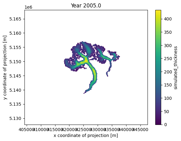
Alternatively, you can create an animation using the merged data, displaying a value every 5 years, as specified above with years_to_merge:
# Get a handle on the figure and the axes
fig, ax = plt.subplots()
thk = ds_merged['simulated_thickness']
# Plot the initial frame.
cax = thk.isel(time=0).plot(ax=ax,
add_colorbar=True,
cmap='viridis',
vmin=0, vmax=thk.max(),
cbar_kwargs={
'extend':'neither'
}
)
ax.axis('equal')
def animate(frame):
ax.set_title(f'Year {float(thk.time[frame]):.1f}')
cax.set_array(thk.values[frame, :].flatten())
ani_glacier = animation.FuncAnimation(fig, animate, frames=len(thk.time), interval=200);
# Visualize
HTML(ani_glacier.to_jshtml())
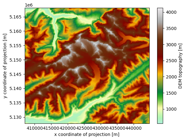
For visualization purposes, the merged dataset also includes the topography of the entire region, encompassing the glacier surfaces:
cmap=salem.get_cmap('topo')
ds_merged.topo.plot(cmap=cmap)
<matplotlib.collections.QuadMesh at 0x7ff464273890>
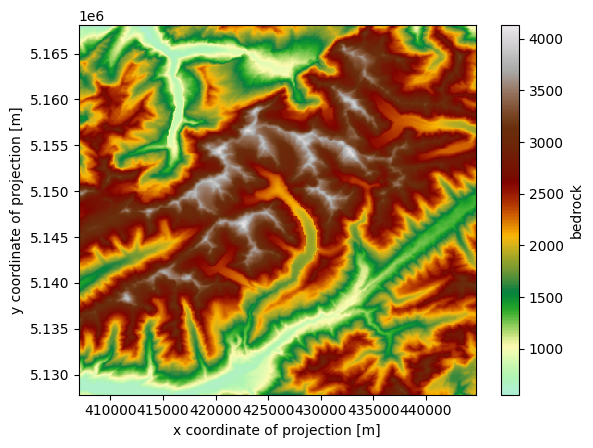
Or the estimated bedrock topography, without ice:
ds_merged.bedrock.plot(cmap=cmap)
<matplotlib.collections.QuadMesh at 0x7ff46416a210>
Nice 3D videos#
We are working on a tool to make even nicer videos like this one:
from IPython.display import Video
Video("../../img/mittelbergferner.mp4", embed=True, width=700)
The WIP tool is available here: OGGM/oggm-3dviz