Compare different DEMs for individual glaciers: RGI-TOPO for RGI v6.0

For most glaciers in the world there are several digital elevation models (DEM) which cover the respective glacier. In OGGM we have currently implemented more than 10 different open access DEMs to choose from. Some are regional and only available in certain areas (e.g. Greenland or Antarctica) and some cover almost the entire globe.

This notebook allows to see which of the DEMs are available for a selected glacier and how they compare to each other. That way it is easy to spot systematic differences and also invalid points in the DEMs.

Input parameters

This notebook can be run as a script with parameters using papermill, but it is not necessary. The following cell contains the parameters you can choose from:

# The RGI Id of the glaciers you want to look for
# Use the original shapefiles or the GLIMS viewer to check for the ID: https://www.glims.org/maps/glims
rgi_id = 'RGI60-11.00897'

# The default is to test for all sources available for this glacier
# Set to a list of source names to override this
sources = None
# Where to write the plots. Default is in the current working directory
plot_dir = f'outputs/{rgi_id}'
# The RGI version to use
# V62 is an unofficial modification of V6 with only minor, backwards compatible modifications
prepro_rgi_version = 62
# Size of the map around the glacier. Currently only 10 and 40 are available
prepro_border = 10
# Degree of processing level.  Currently only 1 is available.
from_prepro_level = 1

Check input and set up

# The sources can be given as parameters
if sources is not None and isinstance(sources, str):
    sources = sources.split(',')

# Plotting directory as well
if not plot_dir:
    plot_dir = './' + rgi_id
import os
plot_dir = os.path.abspath(plot_dir)

import pandas as pd
import numpy as np
from oggm import cfg, utils, workflow, tasks, graphics, GlacierDirectory
import xarray as xr
import rioxarray as rioxr
import geopandas as gpd
import salem
import matplotlib.pyplot as plt
from mpl_toolkits.axes_grid1 import AxesGrid
import itertools

from oggm.utils import DEM_SOURCES
from oggm.workflow import init_glacier_directories

# Make sure the plot directory exists
utils.mkdir(plot_dir);
# Use OGGM to download the data
cfg.initialize()
cfg.PATHS['working_dir'] = utils.gettempdir(dirname='OGGM-DEMS', reset=True)
cfg.PARAMS['use_intersects'] = False

2025-04-16 10:57:09: oggm.cfg: Reading default parameters from the OGGM `params.cfg` configuration file.
2025-04-16 10:57:09: oggm.cfg: Multiprocessing switched OFF according to the parameter file.
2025-04-16 10:57:09: oggm.cfg: Multiprocessing: using all available processors (N=4)
2025-04-16 10:57:09: oggm.cfg: PARAMS['use_intersects'] changed from `True` to `False`.

Download the data using OGGM utility functions

Note that you could reach the same goal by downloading the data manually from https://cluster.klima.uni-bremen.de/data/gdirs/dems_v2/default (high resolution version: https://cluster.klima.uni-bremen.de/data/gdirs/dems_v1/highres)

# URL of the preprocessed GDirs
gdir_url = 'https://cluster.klima.uni-bremen.de/data/gdirs/dems_v2/default'
# We use OGGM to download the data
gdir = init_glacier_directories([rgi_id], from_prepro_level=1, prepro_border=10, prepro_base_url=gdir_url)[0]

2025-04-16 10:57:10: oggm.workflow: init_glacier_directories from prepro level 1 on 1 glaciers.
2025-04-16 10:57:10: oggm.workflow: Execute entity tasks [gdir_from_prepro] on 1 glaciers

Read the DEMs and store them all in a dataset

if sources is None:
    sources = [src for src in os.listdir(gdir.dir) if src in utils.DEM_SOURCES]

print('RGI ID:', rgi_id)
print('Available DEM sources:', sources)
print('Plotting directory:', plot_dir)

RGI ID: RGI60-11.00897
Available DEM sources: ['ASTER', 'COPDEM90', 'AW3D30', 'TANDEM', 'MAPZEN', 'COPDEM30', 'NASADEM', 'SRTM', 'DEM3']
Plotting directory: /__w/tutorials/tutorials/notebooks/tutorials/outputs/RGI60-11.00897

# We use xarray to store the data
ods = xr.Dataset()
for src in sources:
    demfile = os.path.join(gdir.dir, src) + '/dem.tif'
    with rioxr.open_rasterio(demfile) as ds:
        data = ds.sel(band=1).load() * 1.
        ods[src] = data.where(data > -100, np.nan)
    
    sy, sx = np.gradient(ods[src], gdir.grid.dx, gdir.grid.dx)
    ods[src + '_slope'] = ('y', 'x'),  np.arctan(np.sqrt(sy**2 + sx**2))

with rioxr.open_rasterio(gdir.get_filepath('glacier_mask')) as ds:
    ods['mask'] = ds.sel(band=1).load()

# Decide on the number of plots and figure size
ns = len(sources)
x_size = 12
n_cols = 3
n_rows = -(-ns // n_cols)
y_size = x_size / n_cols * n_rows

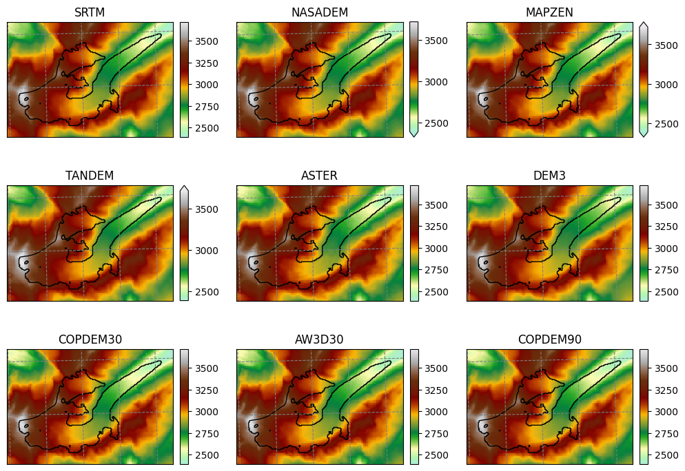
Raw topography data

smap = salem.graphics.Map(gdir.grid, countries=False)
smap.set_shapefile(gdir.read_shapefile('outlines'))
smap.set_plot_params(cmap='topo')
smap.set_lonlat_contours(add_tick_labels=False)
smap.set_plot_params(vmin=np.nanquantile([ods[s].min() for s in sources], 0.25),
                     vmax=np.nanquantile([ods[s].max() for s in sources], 0.75))

fig = plt.figure(figsize=(x_size, y_size))
grid = AxesGrid(fig, 111,
                nrows_ncols=(n_rows, n_cols),
                axes_pad=0.7,
                cbar_mode='each',
                cbar_location='right',
                cbar_pad=0.1
                )

for i, s in enumerate(sources):
    data = ods[s]
    smap.set_data(data)
    ax = grid[i]
    smap.visualize(ax=ax, addcbar=False, title=s)
    if np.isnan(data).all():
        grid[i].cax.remove()
        continue
    cax = grid.cbar_axes[i]
    smap.colorbarbase(cax)
    
# take care of uneven grids
if ax != grid[-1] and not grid[-1].title.get_text():
    grid[-1].remove()
    grid[-1].cax.remove()
if ax != grid[-2] and not grid[-2].title.get_text():
    grid[-2].remove()
    grid[-2].cax.remove()

plt.savefig(os.path.join(plot_dir, 'dem_topo_color.png'), dpi=150, bbox_inches='tight')

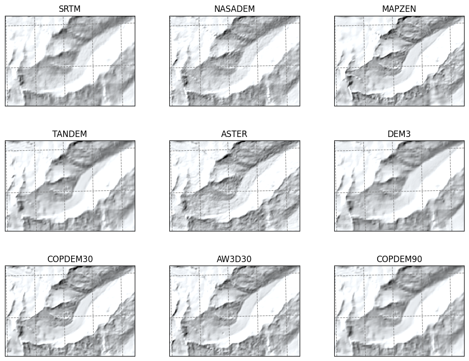
Shaded relief

fig = plt.figure(figsize=(x_size, y_size))
grid = AxesGrid(fig, 111,
                nrows_ncols=(n_rows, n_cols),
                axes_pad=0.7,
                cbar_location='right',
                cbar_pad=0.1
                )
smap.set_plot_params(cmap='Blues')
smap.set_shapefile()
for i, s in enumerate(sources):
    data = ods[s].copy().where(np.isfinite(ods[s]), 0)
    smap.set_data(data * 0)
    ax = grid[i]
    smap.set_topography(data)
    smap.visualize(ax=ax, addcbar=False, title=s)
    
# take care of uneven grids
if ax != grid[-1] and not grid[-1].title.get_text():
    grid[-1].remove()
    grid[-1].cax.remove()
if ax != grid[-2] and not grid[-2].title.get_text():
    grid[-2].remove()
    grid[-2].cax.remove()

plt.savefig(os.path.join(plot_dir, 'dem_topo_shade.png'), dpi=150, bbox_inches='tight')

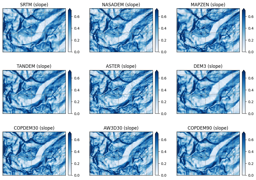
Slope

fig = plt.figure(figsize=(x_size, y_size))
grid = AxesGrid(fig, 111,
                nrows_ncols=(n_rows, n_cols),
                axes_pad=0.7,
                cbar_mode='each',
                cbar_location='right',
                cbar_pad=0.1
                )

smap.set_topography();
smap.set_plot_params(vmin=0, vmax=0.7, cmap='Blues')

for i, s in enumerate(sources):
    data = ods[s + '_slope']
    smap.set_data(data)
    ax = grid[i]
    smap.visualize(ax=ax, addcbar=False, title=s + ' (slope)')
    cax = grid.cbar_axes[i]
    smap.colorbarbase(cax)
    
# take care of uneven grids
if ax != grid[-1] and not grid[-1].title.get_text():
    grid[-1].remove()
    grid[-1].cax.remove()
if ax != grid[-2] and not grid[-2].title.get_text():
    grid[-2].remove()
    grid[-2].cax.remove()

plt.savefig(os.path.join(plot_dir, 'dem_slope.png'), dpi=150, bbox_inches='tight')

Some simple statistics about the DEMs

df = pd.DataFrame()
for s in sources:
    df[s] = ods[s].data.flatten()[ods.mask.data.flatten() == 1]

dfs = pd.DataFrame()
for s in sources:
    dfs[s] = ods[s + '_slope'].data.flatten()[ods.mask.data.flatten() == 1]

df.describe()

	ASTER	COPDEM90	AW3D30	TANDEM	MAPZEN	COPDEM30	NASADEM	SRTM	DEM3
count	3218.000000	3218.000000	3218.000000	3218.000000	3218.000000	3218.000000	3218.000000	3218.000000	3218.000000
mean	3031.316346	3014.512695	3023.871970	3066.820068	3023.202610	3014.124512	3028.332505	3032.272219	3052.045681
std	250.883864	259.186768	253.597569	258.874115	254.144292	259.403259	247.615467	246.447678	237.228101
min	2428.000000	2416.773438	2417.000000	2469.287598	2413.000000	2413.545654	2430.000000	2450.000000	2490.000000
25%	2865.000000	2836.975037	2851.000000	2889.410828	2850.000000	2837.251770	2855.000000	2857.000000	2883.500000
50%	3058.000000	3044.824097	3052.500000	3097.242310	3051.000000	3044.196289	3054.000000	3060.000000	3068.500000
75%	3203.000000	3196.834839	3201.750000	3249.972717	3201.750000	3196.260803	3202.000000	3203.000000	3217.000000
max	3693.000000	3688.330078	3720.000000	3738.977051	3723.000000	3694.253174	3691.000000	3684.000000	3701.000000

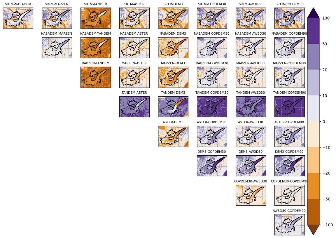
Comparison matrix plot

# Table of differences between DEMS
df_diff = pd.DataFrame()
done = []
for s1, s2 in itertools.product(sources, sources):
    if s1 == s2:
        continue
    if (s2, s1) in done:
        continue
    df_diff[s1 + '-' + s2] = df[s1] - df[s2]
    done.append((s1, s2))

# Decide on plot levels
max_diff = df_diff.quantile(0.99).max()
base_levels = np.array([-8, -5, -3, -1.5, -1, -0.5, -0.2, -0.1, 0, 0.1, 0.2, 0.5, 1, 1.5, 3, 5, 8])
if max_diff < 10:
    levels = base_levels
elif max_diff < 100:
    levels = base_levels * 10
elif max_diff < 1000:
    levels = base_levels * 100
else:
    levels = base_levels * 1000
levels = [l for l in levels if abs(l) < max_diff]
if max_diff > 10:
    levels = [int(l) for l in levels]
levels

[-50, -30, -15, -10, -5, -2, -1, 0, 1, 2, 5, 10, 15, 30, 50]

smap.set_plot_params(levels=levels, cmap='PuOr', extend='both')
smap.set_shapefile(gdir.read_shapefile('outlines'))

fig = plt.figure(figsize=(14, 14))
grid = AxesGrid(fig, 111,
                nrows_ncols=(ns - 1, ns - 1),
                axes_pad=0.3,
                cbar_mode='single',
                cbar_location='right',
                cbar_pad=0.1
                )
done = []
for ax in grid:
    ax.set_axis_off()
for s1, s2 in itertools.product(sources, sources):
    if s1 == s2:
        continue
    if (s2, s1) in done:
        continue
    data = ods[s1] - ods[s2]
    ax = grid[sources.index(s1) * (ns - 1) + sources[1:].index(s2)]
    ax.set_axis_on()
    smap.set_data(data)
    smap.visualize(ax=ax, addcbar=False)
    done.append((s1, s2))
    ax.set_title(s1 + '-' + s2, fontsize=8)
    
cax = grid.cbar_axes[0]
smap.colorbarbase(cax);

plt.savefig(os.path.join(plot_dir, 'dem_diffs.png'), dpi=150, bbox_inches='tight')

Comparison scatter plot

import seaborn as sns
sns.set(style="ticks")

l1, l2 = (utils.nicenumber(df.min().min(), binsize=50, lower=True), 
          utils.nicenumber(df.max().max(), binsize=50, lower=False))

def plot_unity(xdata, ydata, **kwargs):
    points = np.linspace(l1, l2, 100)
    plt.gca().plot(points, points, color='k', marker=None,
                   linestyle=':', linewidth=3.0)

g = sns.pairplot(df.dropna(how='all', axis=1).dropna(), plot_kws=dict(s=50, edgecolor="C0", linewidth=1));
g.map_offdiag(plot_unity)
for asx in g.axes:
    for ax in asx:
        ax.set_xlim((l1, l2))
        ax.set_ylim((l1, l2))

plt.savefig(os.path.join(plot_dir, 'dem_scatter.png'), dpi=150, bbox_inches='tight')

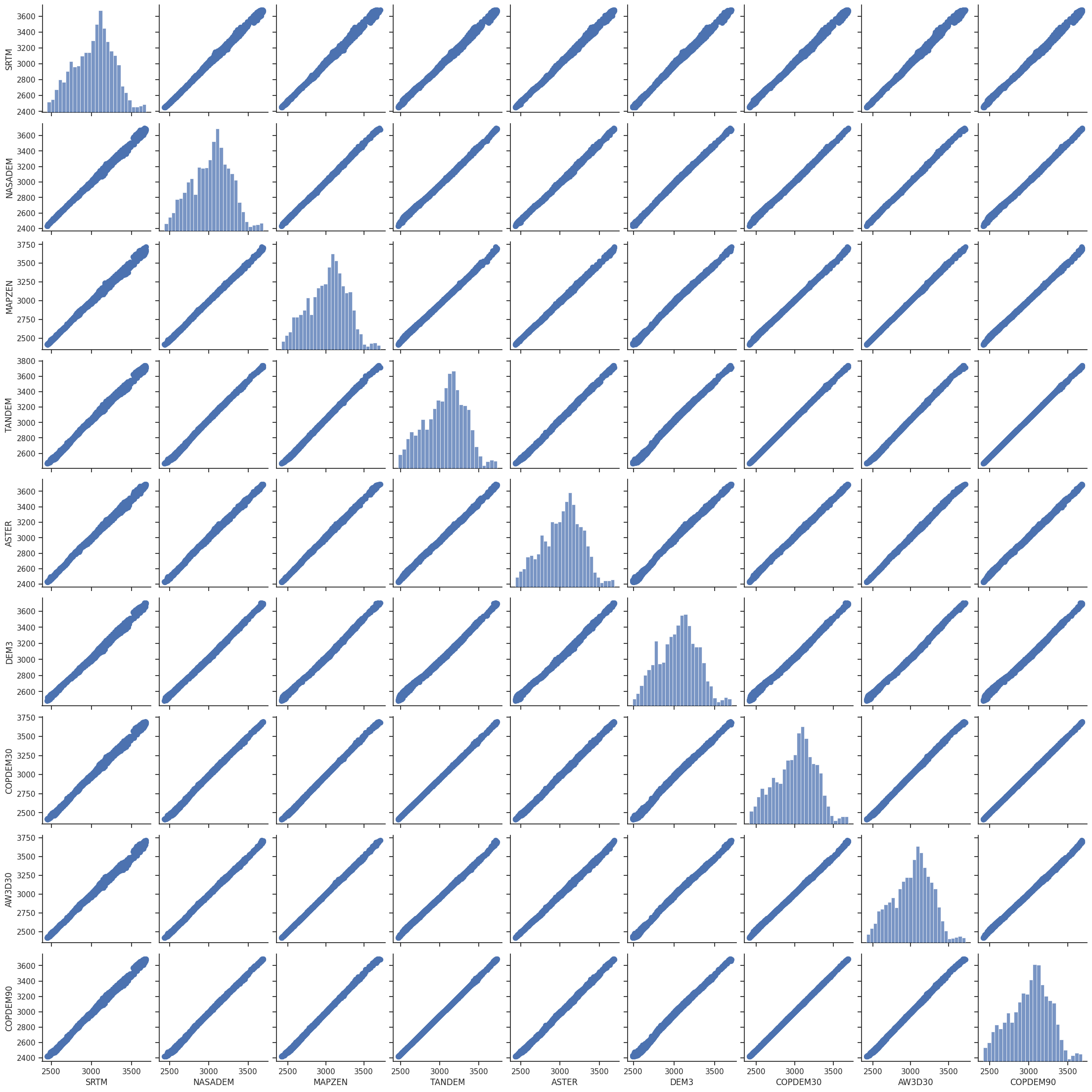
Table statistics

df.describe()

	ASTER	COPDEM90	AW3D30	TANDEM	MAPZEN	COPDEM30	NASADEM	SRTM	DEM3
count	3218.000000	3218.000000	3218.000000	3218.000000	3218.000000	3218.000000	3218.000000	3218.000000	3218.000000
mean	3031.316346	3014.512695	3023.871970	3066.820068	3023.202610	3014.124512	3028.332505	3032.272219	3052.045681
std	250.883864	259.186768	253.597569	258.874115	254.144292	259.403259	247.615467	246.447678	237.228101
min	2428.000000	2416.773438	2417.000000	2469.287598	2413.000000	2413.545654	2430.000000	2450.000000	2490.000000
25%	2865.000000	2836.975037	2851.000000	2889.410828	2850.000000	2837.251770	2855.000000	2857.000000	2883.500000
50%	3058.000000	3044.824097	3052.500000	3097.242310	3051.000000	3044.196289	3054.000000	3060.000000	3068.500000
75%	3203.000000	3196.834839	3201.750000	3249.972717	3201.750000	3196.260803	3202.000000	3203.000000	3217.000000
max	3693.000000	3688.330078	3720.000000	3738.977051	3723.000000	3694.253174	3691.000000	3684.000000	3701.000000

df.corr()

	ASTER	COPDEM90	AW3D30	TANDEM	MAPZEN	COPDEM30	NASADEM	SRTM	DEM3
ASTER	1.000000	0.999365	0.999315	0.999344	0.999455	0.999343	0.999131	0.998518	0.998119
COPDEM90	0.999365	1.000000	0.999660	0.999974	0.999700	0.999958	0.999379	0.998394	0.998282
AW3D30	0.999315	0.999660	1.000000	0.999633	0.999819	0.999679	0.999553	0.998216	0.998638
TANDEM	0.999344	0.999974	0.999633	1.000000	0.999687	0.999932	0.999342	0.998315	0.998220
MAPZEN	0.999455	0.999700	0.999819	0.999687	1.000000	0.999754	0.999643	0.998217	0.998774
COPDEM30	0.999343	0.999958	0.999679	0.999932	0.999754	1.000000	0.999358	0.998275	0.998258
NASADEM	0.999131	0.999379	0.999553	0.999342	0.999643	0.999358	1.000000	0.998544	0.999294
SRTM	0.998518	0.998394	0.998216	0.998315	0.998217	0.998275	0.998544	1.000000	0.997864
DEM3	0.998119	0.998282	0.998638	0.998220	0.998774	0.998258	0.999294	0.997864	1.000000

df_diff.describe()

	ASTER-COPDEM90	ASTER-AW3D30	ASTER-TANDEM	ASTER-MAPZEN	ASTER-COPDEM30	ASTER-NASADEM	ASTER-SRTM	ASTER-DEM3	COPDEM90-AW3D30	COPDEM90-TANDEM	...	MAPZEN-COPDEM30	MAPZEN-NASADEM	MAPZEN-SRTM	MAPZEN-DEM3	COPDEM30-NASADEM	COPDEM30-SRTM	COPDEM30-DEM3	NASADEM-SRTM	NASADEM-DEM3	SRTM-DEM3
count	3218.000000	3218.000000	3218.000000	3218.000000	3218.000000	3218.000000	3218.000000	3218.000000	3218.000000	3218.000000	...	3218.000000	3218.000000	3218.000000	3218.000000	3218.000000	3218.000000	3218.000000	3218.000000	3218.000000	3218.000000
mean	16.803539	7.444375	-35.503534	8.113735	17.191860	2.983841	-0.955873	-20.729335	-9.359164	-52.307072	...	9.078125	-5.129894	-9.069608	-28.843070	-14.208019	-18.147733	-37.921195	-3.939714	-23.713176	-19.773462
std	12.309234	9.720664	12.211383	8.953622	12.572292	10.892745	14.247553	20.258841	8.710851	1.883556	...	7.750302	9.360127	16.809936	20.831143	14.878318	19.706512	26.573851	13.380009	13.812505	18.297883
min	-21.495605	-33.000000	-79.663330	-30.000000	-23.341553	-40.000000	-69.000000	-105.000000	-41.972168	-79.299805	...	-31.172363	-40.000000	-84.000000	-116.000000	-71.462646	-79.334717	-130.334717	-69.000000	-85.000000	-74.000000
25%	8.315002	1.000000	-43.959106	2.000000	8.794128	-3.000000	-10.000000	-27.000000	-14.219543	-52.462891	...	4.448425	-10.000000	-20.750000	-37.000000	-19.370178	-30.145203	-49.488220	-10.000000	-31.000000	-32.000000
50%	14.929077	7.000000	-37.429810	8.000000	15.391968	4.000000	0.000000	-18.000000	-9.151611	-52.428711	...	7.459595	-3.000000	-10.000000	-23.000000	-10.123413	-17.336670	-29.365234	-4.000000	-21.000000	-21.000000
75%	24.004944	13.000000	-28.404724	14.000000	24.869507	9.000000	7.000000	-10.000000	-4.334778	-52.394043	...	11.907959	1.000000	-1.000000	-15.000000	-4.427490	-6.655701	-19.947693	1.000000	-14.000000	-9.000000
max	52.883789	44.000000	0.389160	46.000000	52.308594	55.000000	59.000000	42.000000	29.402100	-23.296631	...	46.652588	51.000000	69.000000	22.000000	27.088867	55.908691	11.646729	59.000000	13.000000	54.000000

8 rows × 36 columns

df_diff.abs().describe()

	ASTER-COPDEM90	ASTER-AW3D30	ASTER-TANDEM	ASTER-MAPZEN	ASTER-COPDEM30	ASTER-NASADEM	ASTER-SRTM	ASTER-DEM3	COPDEM90-AW3D30	COPDEM90-TANDEM	...	MAPZEN-COPDEM30	MAPZEN-NASADEM	MAPZEN-SRTM	MAPZEN-DEM3	COPDEM30-NASADEM	COPDEM30-SRTM	COPDEM30-DEM3	NASADEM-SRTM	NASADEM-DEM3	SRTM-DEM3
count	3218.000000	3218.000000	3218.000000	3218.000000	3218.000000	3218.000000	3218.000000	3218.000000	3218.000000	3218.000000	...	3218.000000	3218.000000	3218.000000	3218.000000	3218.000000	3218.000000	3218.000000	3218.000000	3218.000000	3218.000000
mean	17.410436	9.678682	35.503776	9.781231	17.918605	8.758856	10.924798	22.658484	10.511262	52.307072	...	9.462017	7.451212	15.292107	29.093536	14.978851	22.048134	37.997709	10.136109	23.853014	22.972343
std	11.434442	7.498083	12.210679	7.093540	11.512526	7.128573	9.193391	18.074653	7.278676	1.883556	...	7.276508	7.641868	11.442731	20.479767	14.101744	15.215713	26.464294	9.580093	13.569511	14.072358
min	0.000977	0.000000	0.389160	0.000000	0.000732	0.000000	0.000000	0.000000	0.000977	23.296631	...	0.007568	0.000000	0.000000	0.000000	0.002197	0.003906	0.135986	0.000000	0.000000	0.000000
25%	8.656433	4.000000	28.404724	4.000000	9.204651	3.000000	4.000000	11.000000	5.184937	52.394043	...	4.625854	2.000000	6.000000	15.000000	5.027039	10.525879	19.947693	3.000000	14.000000	12.000000
50%	15.060913	8.000000	37.429810	9.000000	15.604980	7.000000	9.000000	19.000000	9.402832	52.428711	...	7.555664	4.000000	13.000000	23.000000	10.341919	19.279541	29.365234	7.000000	21.000000	22.000000
75%	24.004944	14.000000	43.959106	14.000000	24.869507	12.000000	16.000000	27.000000	14.364990	52.462891	...	12.061157	10.000000	23.000000	37.000000	19.433960	30.630066	49.488220	15.000000	31.000000	32.000000
max	52.883789	44.000000	79.663330	46.000000	52.308594	55.000000	69.000000	105.000000	41.972168	79.299805	...	46.652588	51.000000	84.000000	116.000000	71.462646	79.334717	130.334717	69.000000	85.000000	74.000000

8 rows × 36 columns

What’s next?

• return to the OGGM documentation

• back to the table of contents