Compute smoother centerlines for shapefile output#
This notebook describes how to compute centerlines with OGGM and write them to disk. It is meant for users who are mostly interested in the centerlines, not so much the rest of the OGGM model.
We use an example of a user-provided glacier inventory and DEM (thanks to Liss Andreassen for providing the data).
import rioxarray as rioxr
import geopandas as gpd
import matplotlib.pyplot as plt

from oggm import cfg, utils, workflow, tasks
Data preparation#
Download the demo data. This is a subset of a regional glacier inventory and DEM in Norway:
fpath_inventory = utils.file_downloader('https://cluster.klima.uni-bremen.de/~oggm/tutorials/Norway_Inventory_sel.zip')
fpath_dem = utils.file_downloader('https://cluster.klima.uni-bremen.de/~oggm/tutorials/Norway_DEM_sel.tif')
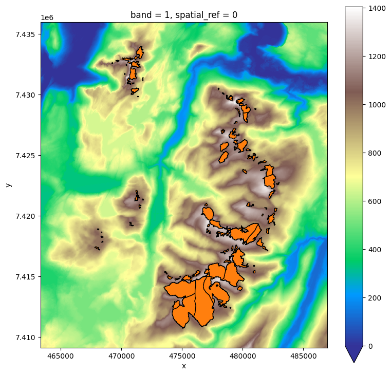
Read the data and plot it:
inventory = gpd.read_file(fpath_inventory)
dem = rioxr.open_rasterio(fpath_dem)

f, ax = plt.subplots(figsize=(9, 9))
dem.plot(ax=ax, cmap='terrain', vmin=0)
inventory.plot(ax=ax, edgecolor='k', facecolor='C1');

The resolution of the DEM is 10m:
print((dem.x[1] - dem.x[0]).item())
10.0
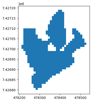
In this inventory, one geometry has a topological error (the figure of eight where the outlines touch):
inventory.loc[~inventory.is_valid].plot();

Let’s correct it:
inventory.loc[~inventory.is_valid, 'geometry'] = inventory.loc[~inventory.is_valid].buffer(0)
A final preparation step is to convert the format of the inventory to a file which resembles the RGI (see use_your_own_inventory.ipynb):
# We keep the original ID for later reference
gdf = utils.cook_rgidf(inventory, o1_region='08', assign_column_values={'breID':'breID'})
Compute the centerlines#
We use the standard OGGM procedure for this:
cfg.initialize(logging_level='WARNING')

# Parameters
cfg.PARAMS['use_multiprocessing'] = True  # this is often a good idea
cfg.PARAMS['use_rgi_area'] = False  # this is required for user-defined inventories
cfg.PARAMS['use_intersects'] = False  # we don't care about intersects for centerlines
cfg.PARAMS['border'] = 10  # no need to make a large map

# Optional: change the grid resolution
# E.g. fixed grid spacing
# cfg.PARAMS['grid_dx_method'] = 'fixed'
# cfg.PARAMS['fixed_dx'] = 10
# Or variable but twice higher than default
cfg.PARAMS['grid_dx_method'] = 'square'
cfg.PARAMS['d1'] = 7  # (default is 14)
cfg.PARAMS['d2'] = 5  # (default is 10)
cfg.PARAMS['dmax'] = 200  # (default is 100)

# Tell OGGM to use our user DEM (important!)
cfg.PATHS['dem_file'] = fpath_dem

# Where to work
cfg.PATHS['working_dir'] = utils.gettempdir(dirname='NORWAY_CENTERLINES', reset=True)
2026-04-11 16:20:05: oggm.cfg: Reading default parameters from the OGGM `params.cfg` configuration file.
2026-04-11 16:20:05: oggm.cfg: Multiprocessing switched OFF according to the parameter file.
2026-04-11 16:20:05: oggm.cfg: Multiprocessing: using all available processors (N=4)
2026-04-11 16:20:05: oggm.cfg: Multiprocessing switched ON after user settings.
2026-04-11 16:20:05: oggm.cfg: PARAMS['use_rgi_area'] changed from `True` to `False`.
2026-04-11 16:20:05: oggm.cfg: PARAMS['use_intersects'] changed from `True` to `False`.
2026-04-11 16:20:05: oggm.cfg: PARAMS['border'] changed from `80` to `10`.
2026-04-11 16:20:05: oggm.cfg: PARAMS['d1'] changed from `14.0` to `7`.
2026-04-11 16:20:05: oggm.cfg: PARAMS['d2'] changed from `10.0` to `5`.
Now the workflow:
gdirs = workflow.init_glacier_directories(gdf)

workflow.execute_entity_task(tasks.define_glacier_region, gdirs, source='USER')  # Use the user DEM

workflow.execute_entity_task(tasks.glacier_masks, gdirs)
workflow.execute_entity_task(tasks.compute_centerlines, gdirs);
2026-04-11 16:20:05: oggm.workflow: Execute entity tasks [GlacierDirectory] on 102 glaciers
2026-04-11 16:20:06: oggm.workflow: Execute entity tasks [define_glacier_region] on 102 glaciers
2026-04-11 16:20:16: oggm.workflow: Execute entity tasks [glacier_masks] on 102 glaciers
2026-04-11 16:20:23: oggm.workflow: Execute entity tasks [compute_centerlines] on 102 glaciers
Note: the default in OGGM is to use a grid size of varying resolution for each glacier. I think it makes sense in many cases, but you may prefer to use the native resolution of your DEM. You can do so by commenting / un-commenting the options above.
Write the data to a shapefile with optional smoothing#
The relevant task is “write_centerlines_to_shape”, which writes everything to a shapefile:
from oggm.utils import write_centerlines_to_shape, mkdir

# We want to write in here
mkdir('outputs')

write_centerlines_to_shape(gdirs,  # The glaciers to process
                           path='outputs/Norway_Centerlines.shp',  # The output file
                           to_tar=False,  # set to True to put everything into one single tar file
                           to_crs=inventory.crs,  # Write into the projection of the original inventory
                           keep_main_only=True,  # Write only the main flowline and discard the tributaries
                           )
2026-04-11 16:20:24: oggm.utils: Applying global task write_centerlines_to_shape on 102 glaciers
2026-04-11 16:20:24: oggm.utils: write_centerlines_to_shape on outputs/Norway_Centerlines.shp ...
2026-04-11 16:20:24: oggm.workflow: Execute entity tasks [get_centerline_lonlat] on 102 glaciers
Let’s have a look at the output:
cls_default = gpd.read_file('outputs/Norway_Centerlines.shp')
cls_default['breID'] = gdf['breID']  # This only works this way because we have one centerline per glacier!

cls_default.head()
| RGIID | SEGMENT_ID | STRAHLER | OUTFLOW_ID | LE_SEGMENT | MAIN | geometry | breID | |
|---|---|---|---|---|---|---|---|---|
| 0 | RGI60-08.00001 | 0 | 0 | -1 | 633.0 | 1 | LINESTRING (471259.347 7433335.143, 471268.347... | 1169 |
| 1 | RGI60-08.00002 | 0 | 0 | -1 | 266.0 | 1 | LINESTRING (471072.559 7433008.446, 471078.622... | 5545 |
| 2 | RGI60-08.00003 | 0 | 0 | -1 | 590.0 | 1 | LINESTRING (470683.14 7432870.887, 470676.217 ... | 1171 |
| 3 | RGI60-08.00004 | 0 | 0 | -1 | 210.0 | 1 | LINESTRING (470772.796 7432860.787, 470766.86 ... | 1170 |
| 4 | RGI60-08.00005 | 0 | 0 | -1 | 293.0 | 1 | LINESTRING (469810.348 7432769.874, 469804.415... | 5546 |
LE_SEGMENT is the length of the centerline in meters. The RGI “IDs” are fake (OGGM needs them) but the breID are real. Let’s use them as index for the file:
cls_default = cls_default.set_index('breID')
orig_inventory = inventory.set_index('breID')
Now we can plot an example:
sel_breID = 1189  # 5570

f, ax = plt.subplots(figsize=(9, 4))
orig_inventory.loc[[sel_breID]].plot(ax=ax, facecolor='lightblue')
cls_default.loc[[sel_breID]].plot(ax=ax);

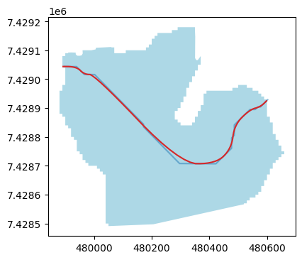
What can we see?
the centerline does not end exactly at the glacier outline
the line seems “crooked”, it has sudden turns
Both effects are due to the algorithm we use to compute the centerlines (Kienholz et al., (2014)), which works on the underlying glacier grid. Each vertice (point) in the line corresponds to the center of the grid point.
We have implemented a few new options in OGGM v1.6, which allow to circumvent these limitations. We illustrate them here:
write_centerlines_to_shape(gdirs,  # The glaciers to process
                           path='outputs/Norway_Centerlines_smooth.shp',  # The output file
                           to_tar=False,  # set to True to put everything into one single tar file
                           to_crs=inventory.crs,  # Write into the projection of the original inventory
                           keep_main_only=True,  # Write only the main flowline and discard the tributaries
                           ensure_exterior_match=True,  # NEW! Ensure that the lines are touching the outlines
                           simplify_line_before=0.75,  # NEW! this option reduces the number of vertices along the line
                           corner_cutting=3,  # NEW! this then augments the number of vertices again
                          )
2026-04-11 16:20:25: oggm.utils: Applying global task write_centerlines_to_shape on 102 glaciers
2026-04-11 16:20:25: oggm.utils: write_centerlines_to_shape on outputs/Norway_Centerlines_smooth.shp ...
2026-04-11 16:20:25: oggm.workflow: Execute entity tasks [get_centerline_lonlat] on 102 glaciers
The simplify_line and corner_cutting options are cosmetic and subjective. The former will simplify the line, by making it look less edgy but also less precise, while the latter then “smoothes” it. Users may try different combinations to see their effect (see the documentation).
cls_smooth = gpd.read_file('outputs/Norway_Centerlines_smooth.shp')
cls_smooth['breID'] = gdf['breID']
cls_smooth = cls_smooth.set_index('breID')
sel_breID = 1189

f, ax = plt.subplots(figsize=(9, 4))
orig_inventory.loc[[sel_breID]].plot(ax=ax, facecolor='lightblue')
cls_default.loc[[sel_breID]].plot(ax=ax, color='C0', alpha=0.5)
cls_smooth.loc[[sel_breID]].plot(ax=ax, color='C3');

Final remarks#
While the centerline algorithm is quite robust, the results will vary as a function of the resolution of the underlying grid, and the smoothing options. After trying a little, it seems difficult to find a setting which works “best” in all circumstances, and we encourage users to try several options and see what they prefer. The option likely to have the most impact (assuming smoothing with (0.5, 5)) is the underlying grid resolution.
What’s next?#
return to the OGGM documentation
back to the table of contents


